- JMP User Community
- :
- Blogs
- :
- JMP Blog
- :
- Predictive models save the day(ta): Well log interpretation and prediction are e...
- Subscribe to RSS Feed
- Mark as New
- Mark as Read
- Bookmark
- Subscribe
- Printer Friendly Page
- Report Inappropriate Content
My favorite class in high school was Earth Science. I recall taking daily weather readings during our meteorology section. Every morning, we went outside, measured wet and dry bulb temperature, wind speed and direction, and estimated cloud cover. Once or twice, we returned to the classroom only to realize a reading was off or didn't make sense. No problem, we went back outside and redid the measurement – it was no big deal to walk the 50 paces and retake the measurement.
The Problem
Fast forward about 18 years, and I am working on the Helix Q4000, attempting to acquire methane hydrate samples from sediment over a mile beneath my feet. It took over 24 hours to acquire our first core. When it came to the surface, nothing had worked properly: The sample was depressurized, and the 10% or so of recovered sediment was just soup. Unlike my temperature readings in high school, we couldn't go back and try again – that sediment sample was forever gone.
This is the challenge geologists and engineers regularly face working in the harsh subsurface environments. The data is expensive to acquire, and you only get one shot. So what do you do when the data doesn't come back as it should? Maybe the tool fails at depth or worse yet, gets stuck and the entire well has to be abandoned? How can we take the little information we have and make useful sense of it? We can use JMP Pro's powerful predictive tools, of course!
The Experiment

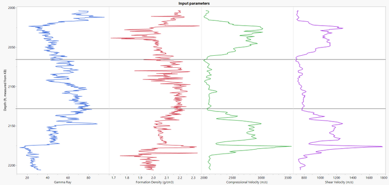
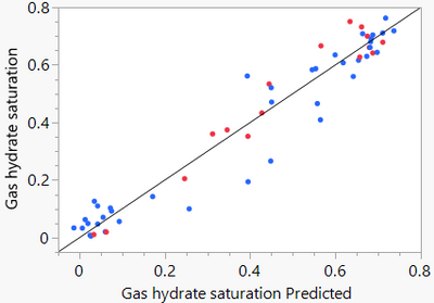
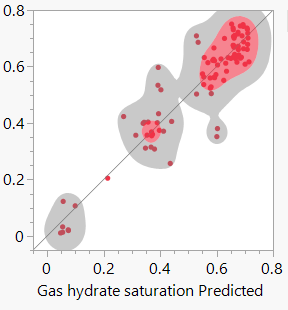
Let's compare a few different methods of predicting a poorly acquired variable from more robust ones. In this instance, we are trying to understand hydrocarbon saturation (methane hydrate), which is sparsely available in this particular well (Mt Elbert well, North Slope, AK). What we do have is complete sets of four variables: Gamma Ray, Formation Density, Compression Velocity, and Shear Velocity. In the subsurface, there are three intervals of hydrate bearing sands, and we want to use the first interval (2003-2064 feet below the kelly bushing, ftkb) to predict hydrate saturation in the lower two intervals, 2065-2127 ftkb and 2128-2206 ftkb, respectively. We will test for different predictive models: Standard Least Squares, Generalized Regression, Neural Network, and XGBoost. We will use R2 values as a first pass of model quality but will then qualitatively evaluate the actual vs. predicted well logs to assess overall quality of each model.
Results

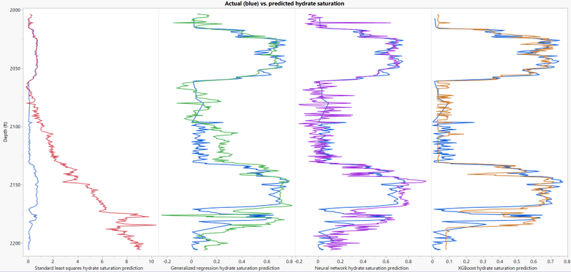
Standard Least Squares just doesn't cut it. It robustly models the Interval 1 but completely fails to predict with any accuracy the hydrocarbon saturation in the lower two intervals. Generalized Regression (Adaptive; Elastic Net) is marginally better but generally overpredicts the lower two intervals by 0.1 to 0.2 saturation units. The machine learning models do a much more robust job, but I give the edge to XGBoost. Neural Network produces a much "noiser" signal in that there are numerous kicks that account for 10-20% over and under prediction, while XGBoost provides a much more stable prediction at both low and high hydrocarbon saturations.
This is a common theme I observe when working with geologic and/or downhole data: The natural systems are incredibly complex, fraught with heterogeneities, and machine learning models (Bootstrap Forest, Neural Network, and XGBoost, etc.) tend to provide better predictive models overall.

Moving Forward
Most folks working in the industry are going to have substantially more data at their fingertips than a single well. A strong practice is to use clustering to group wells together using geologic parameters (lithology, porosity, permeability, etc.) and construct predictive models by cluster. This method can enable you to achieve better outcomes because the model is purpose-built for a particular play, or even a particular basin within a particular play. Beyond that, a great practice is to take a visual walk-about with your data in Graph Builder – try to get a sense of what is going on with individual parameters to identify a best path forward.
Lastly, democratization of data analytics in your organization is going to allow you to achieve greater ends quicker: get powerful tools in user's hands, show them how to build and interpret models, and then sit back and enjoy!
Data Source
This data is was collected through a cooperative agreement drilling between DOE and BP Exploration Alaska (BPXA), in collaboration with the US Geological Survey (USGS) and several universities and industry partners, to evaluate whether natural gas hydrate from the Alaska North Slope could be viably produced either technically or commercially. The Mt. Elbert well was drilled in 2007, and the data is available through the Lamont Doherty Earth Observatory at Columbia University. I subset the data, cleaned it and made it available in a JMP table on JMP Public (Note: Without JMP Pro, the GenReg, Neural w/ KFold, and XGBoost scripts will not execute. Furthermore, the XGBoost script requires JMP Pro and the XGBoost add-in).
You must be a registered user to add a comment. If you've already registered, sign in. Otherwise, register and sign in.
- © 2024 JMP Statistical Discovery LLC. All Rights Reserved.
- Terms of Use
- Privacy Statement
- About JMP
- JMP Software
- JMP User Community
- Contact

