Using functional data as inputs instead of outputs

Jed_Campbell · Sep 19, 2023 10:30 AM

The Functional Data Explorer (FDE) in JMP Pro is generally used when the output of a process is functional/curved data. However, with a few tricks, functional data can also be used as an input to a DOE. To illustrate this, I'll use a fictional case study, walking through the necessary steps along with an explanation of what's happening. I've also attached a JMP journal to this blog post, so readers can follow along.

Background: The ACME Plastic Recycling Company

ACME Plastic Recycling buys bulk shredded plastic, which they melt and form into billets to sell to plastic manufacturers. This shredded plastic comes in different size distributions, which affects the melting process. ACME has created an inexpensive and fast way to get a curve of the size distribution for each incoming shipment. It wants to optimize its melting process parameters to minimize the time needed for each specific shipment.

Step 1: Analyze curve data

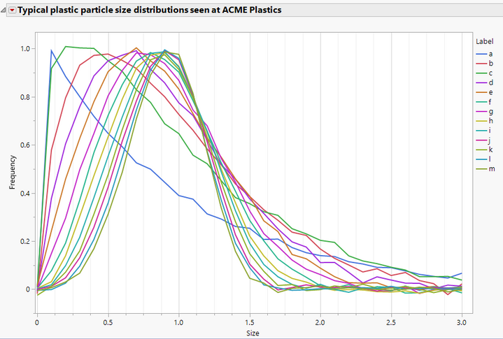
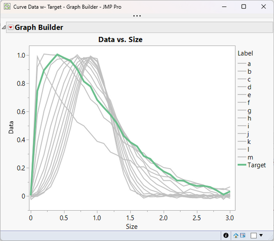
The team created a data set that includes the range of what they generally see for incoming size distributions, which is shown in the graph below:

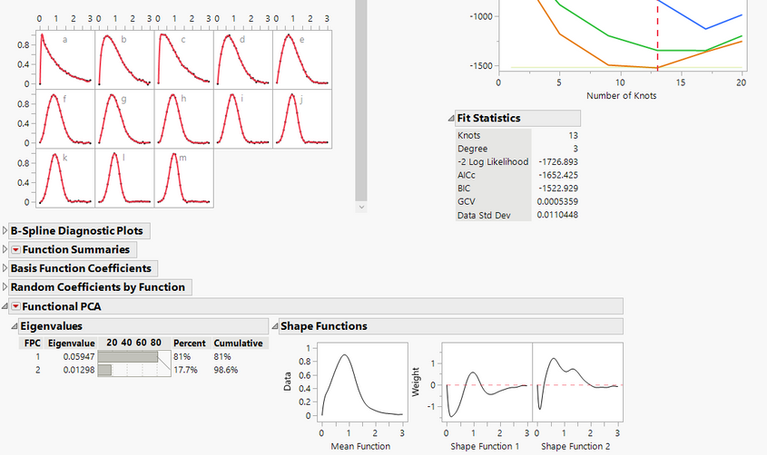
Using the FDE platform, the team found that a simple B Spline with 2 FPCs explains 98.6% of their data. Increasing the FPCs to 3 explains an additional 1%, but adds complexity and runs the risk of trying to predict the noise. They settled on 2 FPCs, as shown below.

2. Output functional principal components

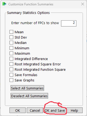
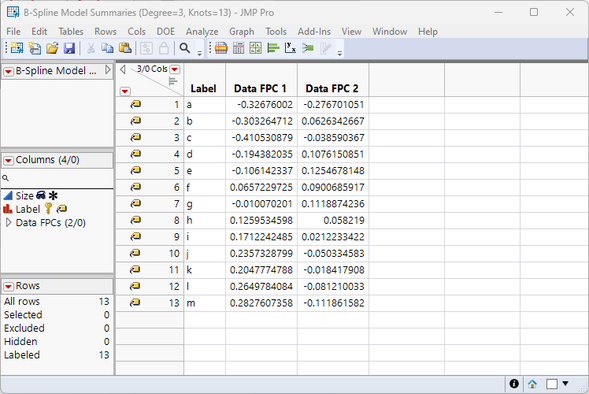
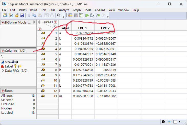
The FDE platform has the ability to output the FPCs from any models that have been fit. This means that the curves, as represented by the FPCs, can be used in other platforms in JMP. Exporting FPCs can be done by selecting the red triangle near the Function Summaries outline, then selecting Customize. Using the "Deselect All" button, then selecting "OK and Save" creates a new data table with the FPCs for each group, as shown in the two images below.

One trick with the data table is needed for later: renaming the "Data FPC 1" and "Data FPC 2" columns to just "FPC 1" and FPC 2" will make linking profilers easier later in the process. Readers who are following along should ensure their data table has updated column names as reflected below.

3. Create and run custom DOE

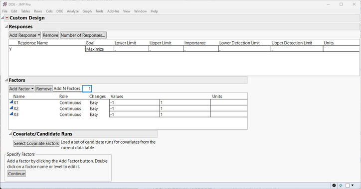
The melting and billeting process has four factors, three of which are continuous, with the fourth being the distribution of the shredded plastic. The team started by using the Custom Designer to populate everything except the distribution of the shredded plastic, as shown below.

The next portion is key: using the FPCs as covariate factors in the Custom Designer forces JMP to use these specific distributions in the experiment. This is possible because each row contains a combination of FPCs, which represent, in this case, 98.6% of all the information in the curves themselves. To accomplish this in the Custom Designer, the team followed these steps:

After making sure the FPC Summary table is the top-most table in the Custom Designer, select Add Factor...Covariate.
In the box that pops up, select the two "Data FPC" columns and hit OK.
After clicking "Continue" and "RSM" to create the model, select the "Allow covariate rows to be repeated" checkbox.
Click "Make Design" to create the experiment and data collection table.

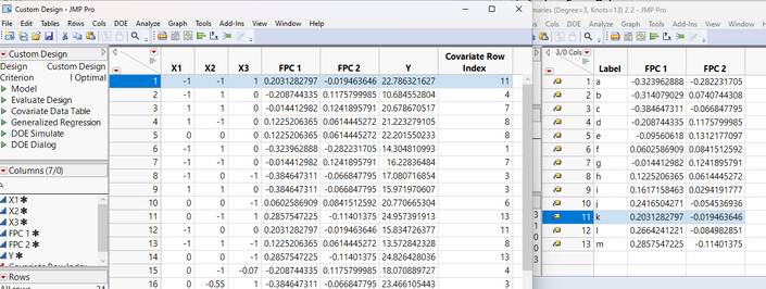
Allowing the covariate rows to be repeated meant that the team needed to find and use raw material that matched the specified distribution. JMP made this easier by including the row number from the FPC data table in the experimental design table. For example, in the screenshot below, the first run used Row 11 from the summaries table, which was the distribution "k" from the original data set used in the FDE platform.

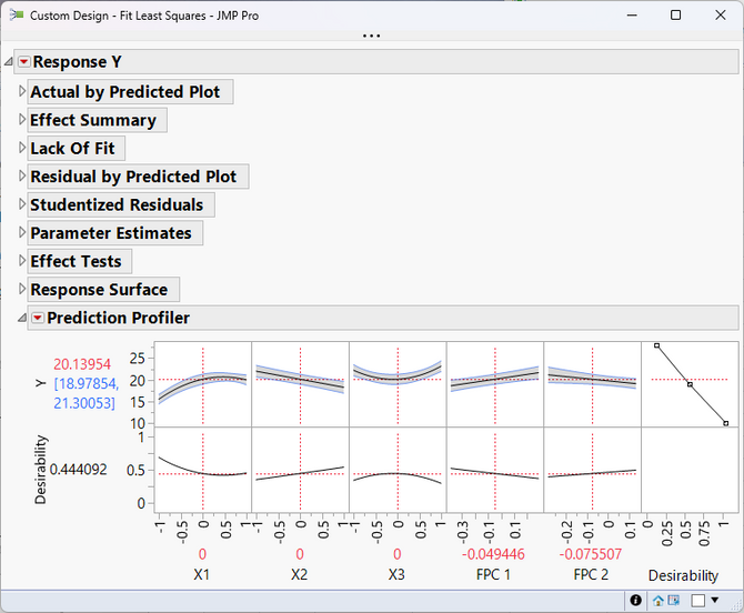
The team completed the experiment with the specified continuous factors (X1 through X3) and the specified plastic size distribution. They then used the model script generated by the Custom Designer, trimming non-significant terms one at a time until only significant terms remained in the model (the "Final Model" script in the journal, for those following along). This model is shown below:

4. Using FDE and Fit Model together

Rather than try to wrap their heads around the FPC 1 and FPC 2 factors in the Prediction Profiler, the team found a simpler method: linking the profilers from the model and the FDE. They did this be selecting the red triangle in the Prediction Profiler...Factor Settings...Link Profilers. Next, they arranged the windows side by side, so changing the FPCs in the Prediction Profiler also changed the curve shape in the FDE window.

Now, the workflow at ACME Plastics has the following steps:

Each new batch has a size distribution performed at the beginning of the process. In the example below, the Target batch doesn't perfectly match any of the previous distributions. This is expected -- it's why the team wanted to use the FDE platform in the first place.

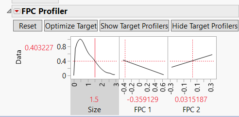
This distribution is input as the Target in the FDE platform, which makes the Optimize Target button available. In this case, the incoming batch is described with FPCs of approximately -.359 and .032.

With the Prediction Profiler from the DOE linked to the FDE platform's FPC Profiler, when the "Optimize Target" button is selected, the Prediction Profiler updates. Locking the two FPCs in the Prediction Profiler then allows the team to maximize desirability for the remaining three continuous factors. In this case, the optimum machine settings are X1 at the low end, X2 at the high end, and X3 set at -0.341.

The team at ACME Plastics has been getting great results with process, and they are now considering taking the excellent and free JSL Scripting course so they can combine the two windows and further streamline their process. For now, they are happy that they are able to use functional data as inputs to their process.